Understanding Flow Matching - A Continuous-Time Generative Framework

Introduction

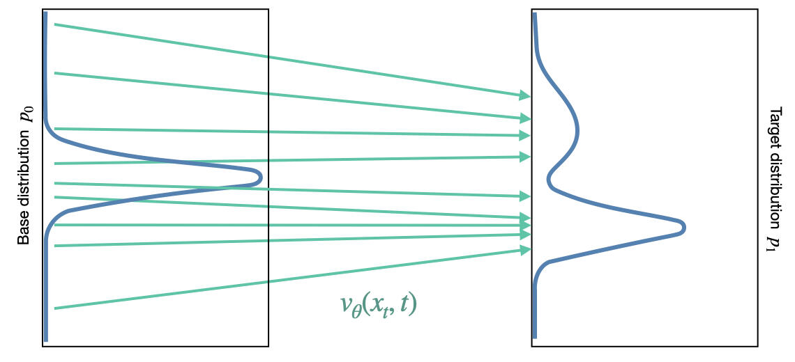
Generative modeling has seen a paradigm shift from the stochastic nature of Diffusion Models to the deterministic elegance of Flow Matching (FM). While Diffusion Models rely on reversing a noise-adding SDE, Flow Matching simplifies the problem by learning a velocity field that pushes a simple noise distribution toward the data distribution along a smooth path.

In this post, we will explore the mathematical framework of Flow Matching and why it is becoming a preferred alternative to traditional diffusion.

Probability Paths and Velocity Fields

Key Definitions and Mappings

To understand Flow Matching, we must first align our physical intuition with mathematical concepts. These concepts are deeply rooted in fluid mechanics and statistical physics.

Concept	Mathematical Symbol	Physical Intuition	Role in Flow Models
Flow Map		The trajectory of a particle (moving an initial point to a destination).	Inference (Sampling): The path from noise to data .
Velocity Field		The speed and direction at every position in space at a given time.	Training Target: The neural network we aim to fit.
Density Field		The concentration of particles (probability density) at each position.	Data Distribution: is noise, is the real data distribution.
Flux Field		The probability mass passing through a unit area per unit time.	Continuity Equation: Describes how probability “flows” through space.

The Continuity Equation: Understanding Flux

The relationship between the density field and the velocity field is governed by the Continuity Equation:

If we define the flux field as , the equation simplifies to:

This is identical to the mass conservation equation in fluid dynamics or the charge conservation equation in electromagnetism:

• is the divergence of the flux, representing how much “probability flow” is exiting (source) or entering (sink) a point.
• is the rate of change of density at that point.
• Physical Meaning: An increase in density at a location () must be balanced by a net inflow of flux (). Probability is neither created nor destroyed.

Main Theory

In Flow Matching, we define a time-dependent probability density for .

• At , is a simple noise distribution (usually standard Gaussian).
• At , is the complex data distribution .

The transformation of samples from to is described by an Ordinary Differential Equation (ODE):

If we know this velocity field, we can generate data by starting with noise and integrating the ODE to find :

The relationship between the probability path and the velocity field is governed by the Continuity Equation:

This equation ensures that the total probability is conserved as the density “flows” from noise to data.

Our goal is to find the velocity field parameterized by a neural network to transfer the simple distribution to the real image distribution .

Conditional Flow Matching (CFM)

If we try to optimize a neural network to match the true velocity field directly using the unconditional continuity equation, we immediately hit a massive computational bottleneck.

Recall that the true time-dependent density field is a marginal distribution obtained by integrating over the entire, intractable data distribution :

Because computing requires integrating over the entire high-dimensional dataset , calculating the ideal unconditional velocity field directly is impossible.

Flow Matching Theorem

To bypass this density bottleneck, we can leverage a beautiful theorem from Flow Matching (Lipman et al., 2022). The core idea is simple: instead of fighting the intractable global distribution, we can break the problem down by conditioning everything on a single, sampled data point .

Theorem:

Let be a chosen conditional probability path, and be its associated conditional velocity field that satisfies the conditional continuity equation:

If we define an aggregate, marginal velocity field by taking a posterior-weighted average of all possible conditional fields:

Then, this is guaranteed to satisfy the unconditional continuity equation for the marginal density .

The Inference Insight: This theorem addresses a fundamental paradox: during training, we can use the knowledge of to construct simple trajectories, but during inference, does not exist. The theorem proves that if a neural network learns to match the conditional fields on average, it will automatically converge to the true, aggregate velocity field needed for generation.

Proof

We want to prove that the defined velocity field satisfies:

From the velocity field we defined above, we will derive to this expression:

Multiply by on both sides:

Take divergence on both sides:

By Leibniz Rule, we can move the symbol inside the integral:

From the conditional continuity equation, we have and plug this into the expression:

Move derivative outside the integral:

The marginal distribution definition is and plug this in:

Finally, we have:

Q.E.D.

Note on Expectation Form: By applying Bayes' rule, we can rewrite the posterior weighting term as . This allows us to express the complex velocity field as a clean, intuitive conditional expectation over the current state:

Optimal Transport Path & Training Objective

To bridge the gap between abstract theory and scalable training, we must choose a specific conditional probability path . Modern flow matching frameworks typically favor the Optimal Transport (OT) Path, which constructs the straightest possible trajectories between noise and data.

There is a subtle but critical distinction between the theoretical definition and the actual implementation variables. Let be the source noise and be a target data point.

Joint Conditioning

When we condition on both the explicit starting point and the final destination , the trajectory is a deterministic linear interpolation:

In this case, the conditional distribution is a Dirac delta function . Taking the time derivative of this path yields the constant velocity vector:

Marginal Conditioning on

To satisfy our main Flow Matching theorem, we must treat the starting point as a distribution instead of a fixed point. Since our trajectory is defined by the linear interpolation , we can derive the strict conditional probability path given only the endpoint as an evolving Gaussian distribution:

At the boundary , this seamlessly simplifies to , perfectly matching our unconditioned standard Gaussian noise. As , the variance collapses to and the distribution sharpens into a Dirac delta function centered exactly at the data point .

By applying the continuity equation to this moving Gaussian bubble, the true Eulerian velocity field reveals a clear spatial dependency:

As the path approaches the data destination (), this formulation suffers from an analytical singularity where we divide by zero. To ensure numerical stability throughout the entire time horizon, we introduce a minor regularizer (e.g., ) to the variance:

Derivation of Particle Path and Regularized Velocity Field

To sample a concrete trajectory point from this modified conditional distribution, we apply the standard Gaussian reparameterization trick. Separating the independent variables of the macro-noise and a static micro-noise yields:

A Note on Boundary Adjustments: It is worth noting that at , this regularized path actually samples from rather than a perfect standard Gaussian. However, because is chosen to be incredibly small, this boundary shift is completely negligible in practice, while the numerical safety it grants at is immense.

Now, substituting our regularized mean and variance into the standard Gaussian transport formula , we resolve the true Eulerian velocity field:

Finding a common denominator and grouping terms containing simplifies the expression into its final, singularity-free formulation:

As , the first term in the numerator vanishes, and the vector field smoothly stabilizes to , preventing any analytical explosion.

Geometric Intuition: Giving the Data Manifold “Thickness”

Beyond fixing the division-by-zero anomaly, the introduction of plays a profound role in smoothing the high-dimensional space.

Real-world datasets concentrate on a low-dimensional sub-space—known as the data manifold—embedded within a massive ambient space. Because this manifold has a lower intrinsic dimensionality, its geometric volume (measure) is strictly zero, behaving like an infinitely thin, sharply folded sheet of paper.

If , the generative flow forces the model to transport noise vectors onto this zero-thickness boundary with absolute precision at . This causes the spatial gradient (Jacobian) of the velocity field to become excessively steep and unstable near the target, introducing optimization friction and causing pixel-level artifacts during generation.

By adding a tiny bit of noise (), we slightly blur each data point. Geometrically, this turns the data from an infinitely thin, sharp surface into a slightly “thickened” layer, making it much easier for the model to learn and generate samples.

This “thickness” acts as a soft-landing pad, allowing simple ODE solvers (like the Euler method) to safely converge with large, discrete step sizes without drifting into unstable space.

Training Objective

While we have derived the exact formulation for the marginal velocity field , directly applying a denominator introduces severe numerical instability during training.

Fortunately, the core Flow Matching theorem provides a beautiful workaround: if we re-introduce the initial noise source as a conditioning variable, the complex conditional velocity field can be simplified into a constant displacement vector. Lipman et al. proved that the marginal conditional field is simply the posterior expectation of the joint conditional field:

Because the neural network minimizes the objective across the entire data distribution, optimizing it to predict the straightforward joint velocity will forces it to automatically converge to the correct, aggregate marginal field in expectation. This completely bypasses the density bottleneck and the division-by-zero anomaly during training.

By using the joint formulation , the expectation over the complex aggregate velocity field simplifies into a straightforward Mean Squared Error (MSE) regression. The neural network simply takes the current interpolated position and time, and predicts the displacement vector:

To address the manifold thickness issue, we can apply a small noise to the interpolated data point:

Sampling Process (Inference)

Generating a new sample is as simple as solving the learned ODE. We start with and solve:

ODE Solvers

Because Flow Matching often learns “straighter” paths than the curved trajectories of diffusion models, we can use efficient ODE solvers:

• Euler Method: The simplest first-order solver.
  

• Higher-order solvers: Methods like RK4 or adaptive step-size solvers (Dormand-Prince) can achieve high accuracy with very few steps.

Compared to Diffusion Models, Flow Matching typically requires significantly fewer steps (e.g., 10-20 steps) to produce high-quality samples.

Conclusion

The brilliance of Flow Matching lies in its ability to bridge the gap between abstract probability densities and concrete particle trajectories. By reformulating generative modeling as a velocity-fitting problem, it replaces the complex stochastic differential equations (SDEs) of diffusion with intuitive, deterministic ordinary differential equations (ODEs).

This shift offers three transformative advantages:

1. Geometric Efficiency: By learning “straighter” paths from noise to data, Flow Matching enables high-quality generation in significantly fewer steps.
2. Mathematical Clarity: The training objective is reduced to a simple MSE regression, removing the need for complex ELBO derivations or variance schedules.
3. Robustness: Techniques like manifold thickening ensure that the model remains stable even when dealing with high-dimensional, complex data.

As we move toward larger and more capable generative systems, Flow Matching provides a cleaner, faster, and more scalable foundation for the next generation of AI.